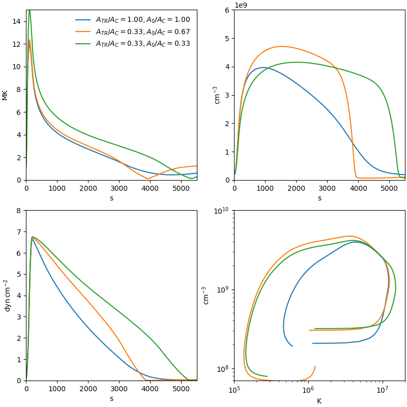
The Effect of Cross-sectional Area Expansion

In this example, we demonstrate the effect of expanding cross-sectional area on the time-evolution of the temperature, density, and pressure. We will reproduce Figure 7 of Cargill et al. [CBKB22].

import astropy.units as u
import matplotlib.pyplot as plt

from astropy.visualization import quantity_support

import ebtelplusplus

from ebtelplusplus.models import HeatingModel, PhysicsModel, TriangularHeatingEvent

quantity_support()

<astropy.visualization.units.quantity_support.<locals>.MplQuantityConverter object at 0x7890e8ed1fa0>

In ebtelplusplus, cross-sectional area expansion is defined through two ratios: the ratio between the cross-sectional area averaged over the transition region (TR) to the cross-sectional area averaged over the corona (\(A_{TR}/A_C\)) and the ratio between the cross-sectional area at the TR-corona boundary and the cross-sectional area averaged over the corona (\(A_0/A_C\)). An additional third parameter, \(L_{TR}/L\), the ratio between the length of the TR and the loop half-length, controls the thickness of the TR.

We will explore the effect of three different expansion profiles: no expansion, gradual expansion from the TR through the corona, and rapid expansion in the corona.

We start by defining our simple single-pulse heating model that we will use in all three cases. Note that we will use a heating partition of \(1/2\) because we will assume a single fluid model in this case to be consistent with Cargill et al. [CBKB22].

heating = HeatingModel(background=3.5e-5*u.Unit('erg cm-3 s-1'),
                       partition=0.5,
                       events=[TriangularHeatingEvent(0*u.s, 200*u.s, 0.1*u.Unit('erg cm-3 s-1'))])

Next, we will set up our three expansion models following Cargill et al. [CBKB22]. In all cases except the no expansion case, we set \(L_{TR}/L_C=0.15\) to model a TR with a small, but finite thickness.

no_expansion = PhysicsModel(force_single_fluid=True)
gradual_expansion = PhysicsModel(force_single_fluid=True,
                                 loop_length_ratio_tr_total=0.15,
                                 area_ratio_tr_corona=1/3,
                                 area_ratio_0_corona=2/3)
coronal_expansion = PhysicsModel(force_single_fluid=True,
                                 loop_length_ratio_tr_total=0.15,
                                 area_ratio_tr_corona=1/3,
                                 area_ratio_0_corona=1/3)

Now, run each simulation for a loop with a half length of 45 Mm for a total simulation time of 5000 s.

loop_length = 45 * u.Mm
total_time = 5500 * u.s
r_no_expansion = ebtelplusplus.run(total_time, loop_length, heating=heating, physics=no_expansion)
r_gradual_expansion = ebtelplusplus.run(total_time, loop_length, heating=heating, physics=gradual_expansion)
r_coronal_expansion = ebtelplusplus.run(total_time, loop_length, heating=heating, physics=coronal_expansion)

Finally, let’s visualize our results in the manner of Figure 7 of Cargill et al. [CBKB22].

fig, axes = plt.subplot_mosaic(
    """
    TN
    PO
    """,
    figsize=(8,8),
    layout='constrained',
)
for result, model in [(r_no_expansion, no_expansion),
                      (r_gradual_expansion, gradual_expansion),
                      (r_coronal_expansion, coronal_expansion)]:
    label = f'$A_{{TR}}/A_C={model.area_ratio_tr_corona:.2f},A_0/A_C={model.area_ratio_0_corona:.2f}$'
    axes['T'].plot(result.time, result.electron_temperature.to('MK'), label=label)
    axes['N'].plot(result.time, result.density)
    axes['P'].plot(result.time, result.electron_pressure+result.ion_pressure)
    axes['O'].plot(result.electron_temperature, result.density)
axes['T'].legend(frameon=False,loc=1)
for ax in ['T','N','P']:
    axes[ax].set_xlim(0,5500)
axes['T'].set_ylim(0,15)
axes['N'].set_ylim(0,6e9)
axes['P'].set_ylim(0,8)
axes['O'].set_xlim(1e5,2e7)
axes['O'].set_ylim(7e7, 1e10)
axes['O'].set_xscale('log')
axes['O'].set_yscale('log')